Activity 5 - Area Estimation of Images with Defined Edges

One of the most helpful information from image processing is the area or size estimation. Usually, images for research, or other data acquiring activities make sure that there is an object with known scale included in the picture. This is for us to know the actual size of a desired object in the image.

Obviously, one can measure the area of an image, by using the measurements provided by a RULER (a real one or from a document/image processing program, and then calculation by brute force.

The activity aims to be able to measure an area of a given figure/image, using image processing tools without having to resolve to tedious calculations. In this note we utilize the the derived discrete form of Greens Theorem given by the following equation [1]

 

where Nb is the total number of pixels in the boundary or contour of the area.[1]

To start this activity, we again use the codes in scilab previously discussed in Activity 4 to create different shapes like we did in Activity 2.

nx = 500; ny = 500; //defines the number of elements along x and y
x = linspace(-1,1,nx); //defines the range
y = linspace(-1,1,ny);
[X,Y] = ndgrid(x,y); //creates two 2-D arrays of x and y coordinates

//Centered Circle
r = sqrt(X.^2 + Y.^2); //note element-per-element squaring of X and Y
image1 = zeros (nx,ny);
image1 (find(r<0.3) ) = 1;
imshow(image1);
imwrite(image1,'C:\Users\GreyFOX\Desktop\Activity5\circle.bmp');

// Centered Square
image2 = zeros(nx,ny);
r = (abs(X+Y) + abs(X-Y));
image2 (find(r<0.4) ) = 1;
imshow(image2);
imwrite(image2,'C:\Users\GreyFOX\Desktop\Activity5\square.bmp');

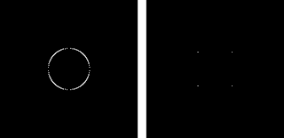
The previous code, produces image1 - a circle, and image2 - a square. Obviously the theoretical area of the is calculated as 0.2642 given that r = 0.29 from the code; while the area of the square is known to be 0.16 given the arbitrary unit of the matrix space.

Figure 1. Image with areas to be measured

circle1 = imread('C:\Users\GreyFOX\Desktop\Activity 7\circle.bmp');
square1 = imread('C:\Users\GreyFOX\Desktop\Activity 7\square.bmp');

edges = edge(circle1, 'sobel'); \\ 'sobel' can be varied 
imwrite(edges,'C:\Users\GreyFOX\Desktop\Acitivity 7\sobel.bmp'); \\the filename is also varied according to the edge method
imshow(edges);

With the predefined images(figure 1), the previous code is used to detect the edges of both images. Consequently, there are different types of edge methods in scilab. Using the help function in scilab and finding edge in it. I obtained the following description.

Figure 2. Description 

Figure 3. Edge using sobel method

Figure 4. Edge using prewitt method

Figure 5. Edge using log method

Figure 6. Edge using fftderiv method

Figure 7. Edge using canny method

For me, i think the best method would be the 'fftderiv' method with a defined edges, compared to 'sobel' and 'canny' which we could see that there are some undefined or blurred parts. On the other hand, the 'log method' produced very thick edges that may affect the area calculation.

Given these images of the edges of the areas were calculated using the derived discrete form of Green's theorem implemented by the following code. Take note that these codes are continuous with the previous codes, meaning circle1 is the previously created circle in figure 1a.


After having the edge determined by the function edge() in scilab, the following code's algorithm is as follows.
1)Find the pixel coordinate of the entire edge
2)Sort these with increasing angle
3)Convert to polar coordinates r and theta
4)Sort [x,y] pairs to increasing theta

Given these contour data, we implemented the greens function using the for loop in the code.
The last part just displays the results and convert it to an arbitrary unit

edges = edge(circle1, 'sobel');

[i,j] = find(edges);
yc = sum(i)/length(i);
xc = sum(j)/length(j);

y = i-yc;
x = j-xc;

theta = atan(y,x);

[theta, k] = gsort(theta, 'g', 'i');
r = sqrt(x**2+y**2);

SUMMATION = 0;
i($+1) = i(1);
j($+1) = j(1);
k($+1) = length(theta)+1;

for l = 1:length(theta)
    SUMMATION = SUMMATION + i(k(l+1))*j(k(l)) - i(k(l))*j(k(l+1));
    //greens function
end
Area = 0.5*SUMMATION;

disp(Area);

realarea = Area*(0.004**2)
disp(realarea);

Using these, I compared the percent deviation of the calculated area with the theoretical value given beforehand.

Table 1. %Deviation of results

As we can see, the method fftderiv is better than the others, one may use these methods with their interest. Maybe the sobel method can detect corners of other shapes and may be helpful to someone.

Using the best method based on the results, which is the fftderiv, I used this to calculate the area of The Bahay ng Alumni in UP Diliman, viewed by a satellite from google maps. I choose these place with known area around 3000 sqm. [2]

Using the scale at the bottom right, I found out that it has 35 pixels for every 10m. I did this by noting the pixel coordinate of the scale.

Figure 9. Area of The Bahay ng Alumni

Using the same algorithm, and 'fftderiv' edge method the calculated area is 2824.081632653061 m^2. I already converted it using the conversion from pixel area to meters which is already presented. It yielded 5.8639% deviation to the estimated area of The Bahay ng Alumni

-------------------------------------------------
I would give myself a grade of 11/10 for i produced all the necessary outputs as well as observe different methods of the edge() function. I also was able to calculate with a good accuracy an area given a map using the knowledge i learned.

References:
[1]AP 186 Handouts. A2 – Area Estimation for Images with Defined Edges. Maricor Soriano 2013
[2] http://www.upalumni.ph/wp-content/uploads/2013/06/rates-new.pdf

Acknowledgements:
Thanks to Tor (Bareza), for helping me understand pixel to other unit conversion which lead me to finish this activity. Also thanks to Ate Bastine (Carpio) for helping me understand scilab matrix and operations.